What’s It Worth?
The pros and cons of different valuation methods
Hi reader,
I tend to get plenty of questions related to the different valuation methods I use every time I share a valuation exercise, so I thought it would be a good idea to write an article describing the most widely used valuation methods and their pros and cons (at least how I see them). At the end of the article, I will also share my preferred valuation method, which many of you might already be familiar with (spoiler: it also has drawbacks).
What’s important to understand is that the ultimate goal of any of these valuation methods is the same: to understand how much a given asset (a company, in this case) is worth. I should also note that the underlying drivers of all these methods I am about to share are also the same, with the only difference being how explicitly/implicitly they are shown. For example, a valuation multiple implies a certain terminal growth rate, even if it’s not explicitly stated like it is when building a Discounted Cash Flow model. In one way or another, every valuation method is discounting future cash flows to the present.
Let’s start with the most widely used valuation method of all (unfortunately).
1. Historical multiples
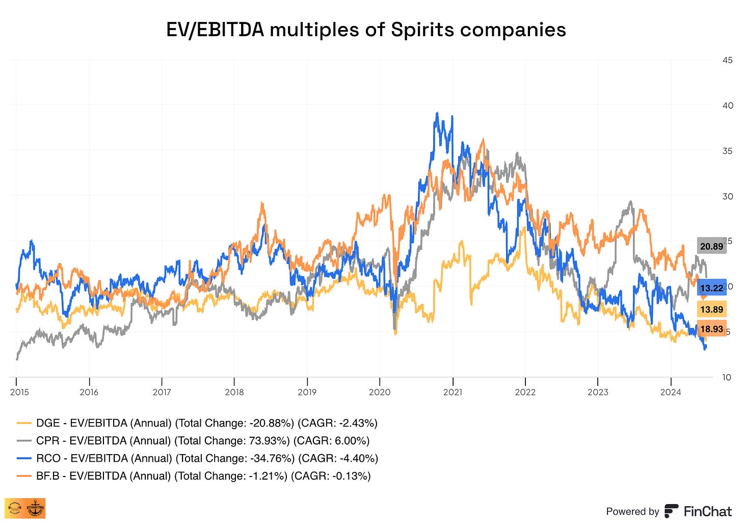
I named this section “Historical Multiples,” although I acknowledge that multiples can be used both for comparisons with the present and the past. When comparing to the present, people typically use multiples to compare different companies in a given industry (i.e., comparisons across peers). For example, I can “easily” compare the EBITDA multiples of the different spirits companies:
(Talking about spirits, I recently released a podcast episode on the industry with Christian Billinger, where we go over all the important things. You can also read my Diageo deep dive if interested)
The problem with such a comparison is that it leads many to think that a given company is relatively cheaper when trading at a lower multiple than a direct peer, which may or may not be true. And that’s precisely one of the main drawbacks here: multiples are too simplistic and don’t explicitly state the underlying drivers of shareholder value creation. Despite many believing that growth is the only variable that matters in a multiple, there’s much more to the story, and I’d go as far as to say that growth over the next 5 years is not even one of the top 2 things to consider in a valuation exercise (albeit it matters). For a quick guide of what multiples imply, you can read this article I wrote a while ago (but wait until you finish this one).
Three other drawbacks of using multiples to compare peers are that…
We must know what the appropriate multiple is for any given industry. For example, I think FCF multiples adjusted for SBC are more appropriate for software companies than P/E multiples because negative working capital is an inherent characteristic of their business model.
The companies that we are comparing must follow almost identical accounting methods, and if they don’t, we must adjust the metrics to make comparisons fair.
Accounting numbers must be normalized.
As you can see, right out of the bat, we get around 4 drawbacks but only one advantage: it’s quick. Unfortunately for investors, a fast arrival to a conclusion is unlikely to compensate for inaccurate information. Sure, multiples are a fast and simple way of getting a first opinion, but more work is needed.
Another thing several people do is compare today’s multiples to those of the past for a given company. The goal of this method is to understand if a company is over or undervalued compared to its history. For example, if I compare Adobe’s current P/FCF ratio with its 10-year average, I could argue that the company is currently slightly overvalued. I reached this conclusion in a matter of seconds, and if I were to upload this to X (formerly Twitter), I would most likely get quite a bit of engagement:
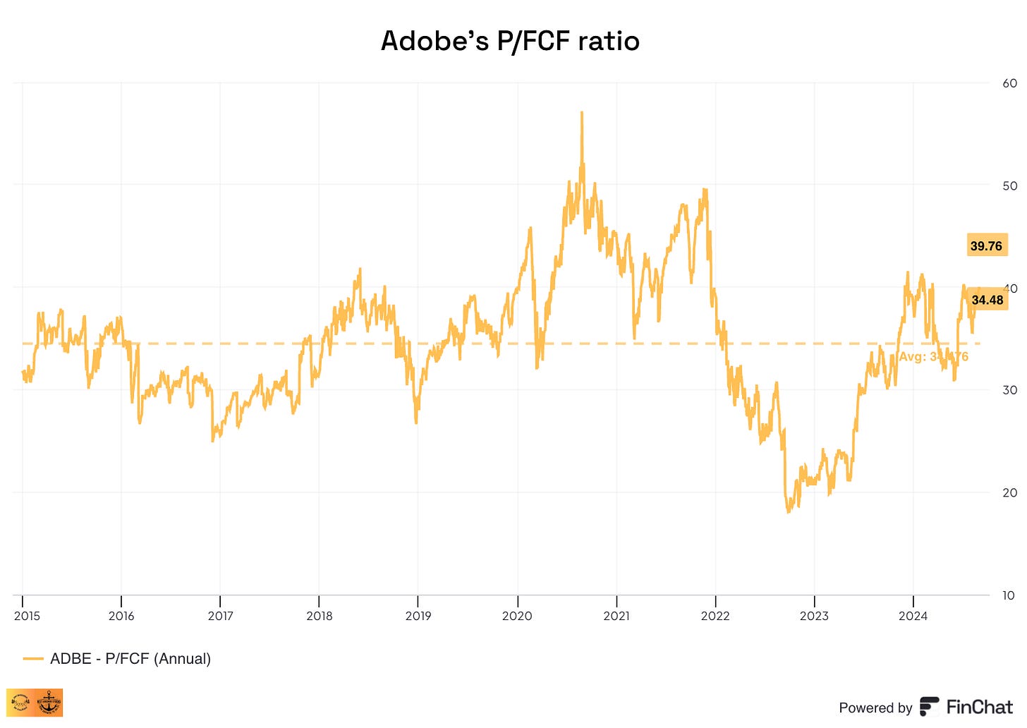
However, as you rightly imagined, this method can lead investors to extremely misleading conclusions for several reasons.
For starters, the underlying company might have changed a fair bit through the years, and we would be completely ignoring this transformation in our valuation exercise. Continuing with the Adobe example…10 years ago, the company was a primarily product-led (not subscription) business. With 90%+ of its revenue today being subscription-like, it makes little sense to compare its multiple today to the one it had in the past.
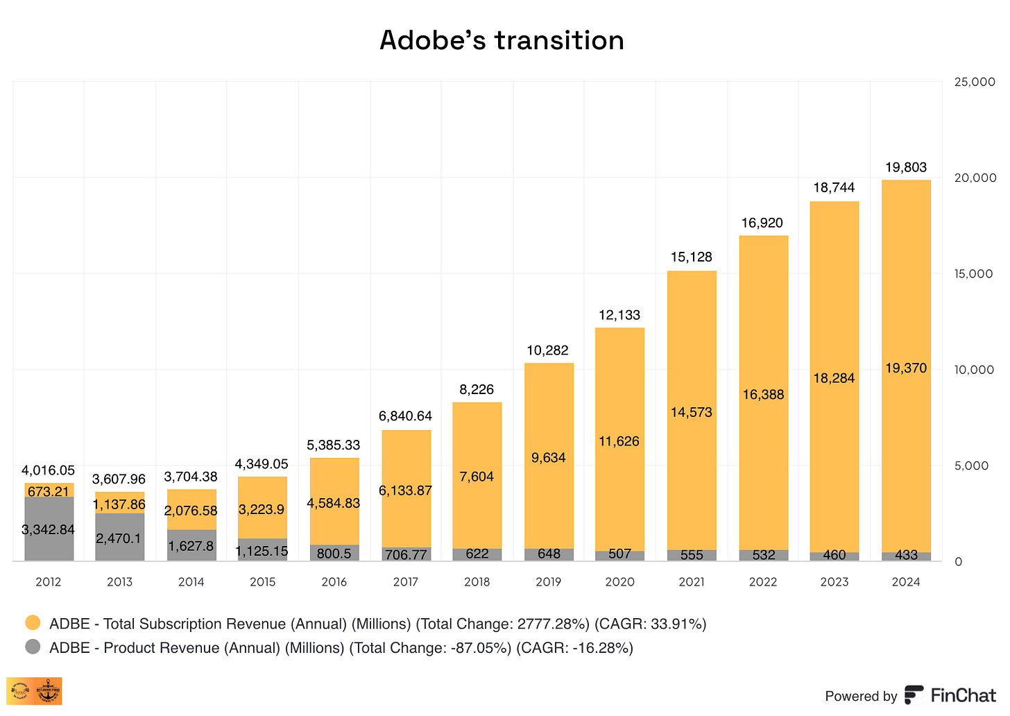
All things equal, subscription revenue should be valued higher by the market than product-based revenue due to its resilience and predictability. Of course, there are other nuances here. For example, it would be logical to think that Adobe’s growth runway today is less significant than its growth runway 10 years ago, but on the other hand, Adobe’s margins are higher. All of these nuances are not explicitly stated when using historical multiples because the efficacy of this method relies on ceteris paribus (i.e., on all other variables remaining constant). Ceteris paribus, however, is tough to apply in a complex world over long periods.
Another good example here is Danaher, which has transitioned from an industrial business to a life sciences-focused company. It’s also now much more focused on organic growth than inorganic growth (something the market typically values higher).
The other drawback when using historical multiples stems from the concept of justified multiples. Justified multiples are calculated in hindsight and show what multiple an investor could’ve paid for a company to realize a market-like return. If a company has outperformed in the past, its justified multiple will be higher than its reported multiple. Conversely, if a company has underperformed in the past, its justified multiple will be lower than its reported multiple. Both of these scenarios basically mean that if a company has out/underperformed in the past, then past reported multiples are, in essence, misleading. Constellation Software is a good example here because it has enjoyed a total return CAGR of 34% over the last decade, making all past multiples extremely misleading:
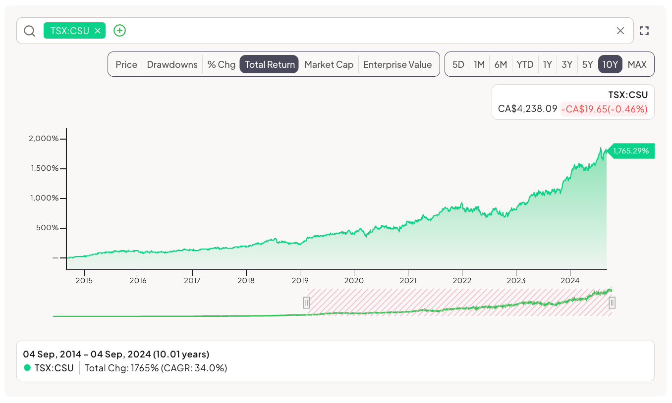
The reason is that the market was not valuing Constellation appropriately in the past, or else it would’ve compounded at a market-like return or maybe slightly higher considering its “higher” risk (i.e., risk-adjusted returns should’ve been the same as the overall market). This is something I touched on in a recent article on Constellation:
Over the last 10 years, the S&P 500 has returned a 12.6% CAGR, whereas Constellation has returned a 33% CAGR. The company traded at 17x OCF back then, but what multiple would’ve made Constellation achieve a market-like return? Constellation was trading at $251 back then, and it’s currently trading at close to $3,000 (all these numbers in USD). To achieve a 12.6% return like the market, an investor could’ve paid up to $900 for Constellation, putting the company trading at an OCF multiple of 61 times 10 years ago! Note that this is not numerically precise because I am ignoring dividends. It’s simply an exercise to show how misleading historical multiples can be, especially since, for winning companies, they are typically below what they should’ve been.
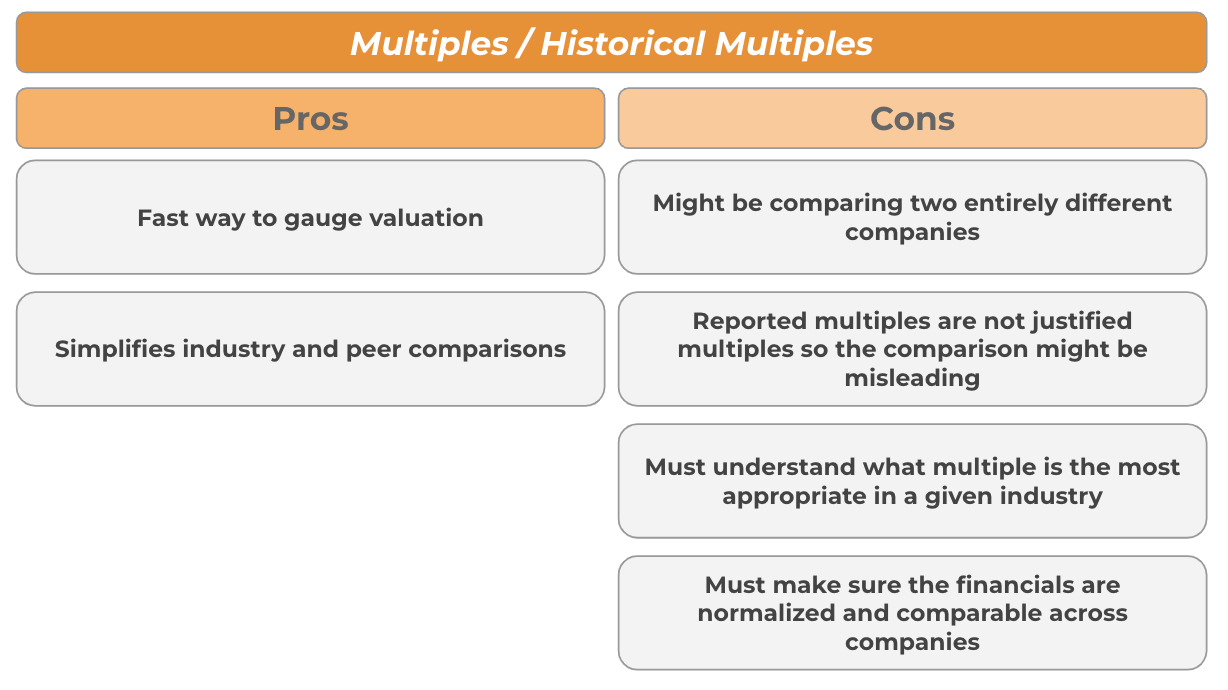
So, in short, while using current and historical valuation multiples might be a fast and quick way (and many people’s preferred way) of judging valuation, it’s a method that has significant drawbacks; there’s simply no shortcut to valuation (or else we would all be rich). Here’s a summary of the pros and cons I see here:
2. FCF and Earning yields
Looking at earnings and FCF yields is basically looking at the inverse of valuation multiples; they are two sides of the same coin. For example, a company trading at a P/E multiple of 20x has an earnings yield of 5% (1/20 = 0.05). Similarly, a company trading at a P/FCF multiple of 30x will be trading at a FCF yield of 3.33% (1/30 = 0.033). The higher the multiple, the lower the yield. This inverse relationship becomes pretty evident if we look at it graphically…
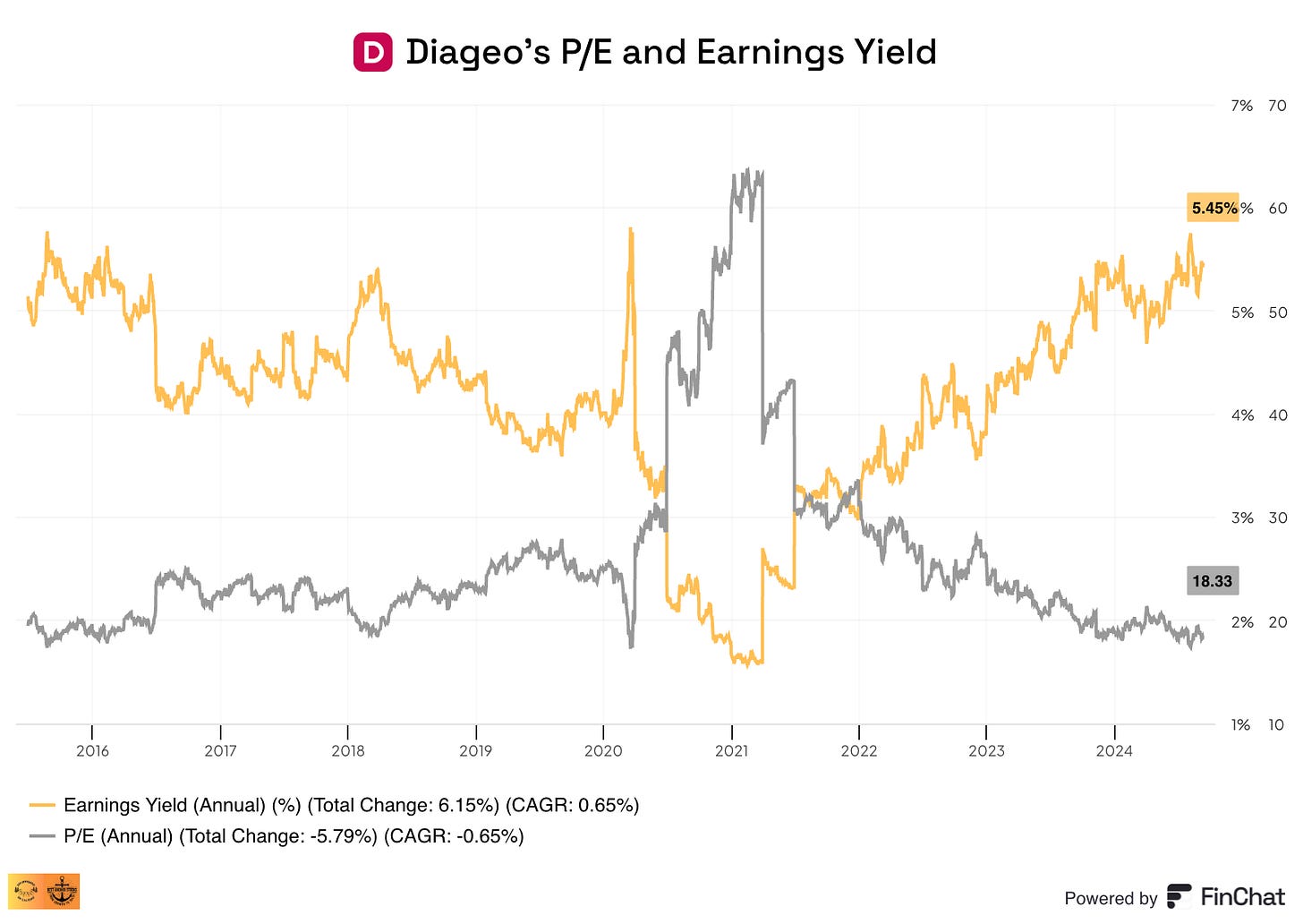
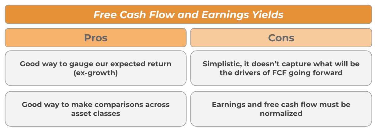
Despite both numbers being pretty much equivalent, I do think that yields possess some advantages compared to multiples. Firstly, it allows us to better understand the return we are getting. If a company is trading at a FCF yield of 5%, this means that if we assume no growth going forward then we should expect a 5% return on our investment (obviously, this also assumes the business doesn’t shrink and that all FCF is paid out to shareholders).
This method also makes comparisons across asset classes easier because I can directly compare the yield of a stock with that of a bond (something that’s quite tough while using multiples because bonds don’t trade at multiples of earnings).
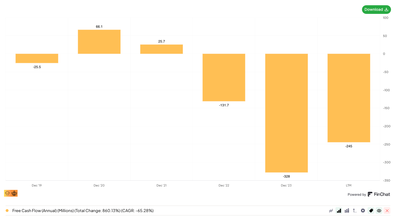
This leads me to the next point: we should be careful comparing stock yields with those of bonds for many reasons, but maybe the most important one is that stocks have embedded a certain level of growth (some do not, but those are not the object of this article), while bonds do not grow their “earnings.” This means that if we directly compare the yield of a stock with that of a bond we are comparing the yield of a growing asset with that of a no-growth asset. Most businesses reinvest part of their earnings to grow, so their FCF and earnings yields tend to be penalized by these investments. For example, this is a company that I am currently looking at (not showing the name, but I’ll write about it at some point). This company has recently invested +$400 million in Capex, of which 92% is growth Capex. This has taken the FCF figures into negative territory, so it would be obviously unfair to compare the FCF yield of this company with that of a bond to judge whether it’s a good opportunity:
A better way to compare these assets is to look at the FCF yield ex-growth, something that I discussed in this article, using the example of Copart. This concept is somewhat similar to Warren Buffett’s “owner earnings.” As per Berkshire’s 1986 shareholder letter:
These represent (a) reported earnings plus (b) depreciation, depletion, amortization, and certain other non-cash charges such as Company N's items (1) and (4) less ( c) the average annual amount of capitalized expenditures for plant and equipment, etc. that the business requires to fully maintain its long-term competitive position and its unit volume. (If the business requires additional working capital to maintain its competitive position and unit volume, the increment also should be included in (c)
Owner earnings can be understood as the earnings of a business minus the expenses required to keep it running at a current state. Free Cash Flow minus maintenance Capex is not a perfect proxy, but it is a good approximation. I say it’s not a perfect proxy because it’s likely that a company needs a slightly higher level of Capex than maintenance Capex to remain competitive (i.e., not shrink) today.
Anyway, going back to this topic, I tend to use the FCF yield to make a quick approximation of my future returns. This is the formula I use:
FCF yield + Expected FCF growth = My expected return
Of course, this formula has some drawbacks, the main ones being that it doesn’t assume any multiple expansion/contraction whatsoever, assumes that all Free Cash Flow is returned to shareholders, and assumes current FCF is normalized.
The math behind it is quite simple. If a stock is trading for $100 and trading at a 5% FCF yield (so generating $5 in FCF per share) and is expected to grow its FCF at a 10% clip, then I should expect to make the 5% in FCF yield and the stock should appreciate 10% if the multiple doesn’t expand or contract. This should lead me to (approximately) a 15% total return on my investment.
Obviously, this is not entirely realistic because multiples don’t tend to remain static, and we should expect them to move (generally down but maybe up, depending on the circumstances). For this reason, this method is useful in…
Situations where the multiple is unlikely to contract significantly or where an expansion is most likely
Situations where the formula above results in a significant margin of safety and where multiple contraction will not make or break or future returns
Going back to the comparability of this method with the one I discussed above, it also suffers the additional drawback that the FCF figure must be normalized, something that’s rarely the case considering how many variables play a role in determining Free Cash Flow. Free Cash Flow is impacted by margins, cash conversion, and Capex, so if any of these variables is not normalized, neither will Free Cash Flow:
3. The Discounted Cash Flow model (aka, DCF)
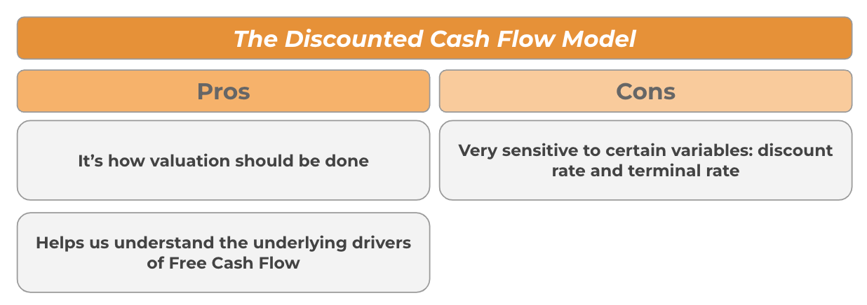
This method is the holy grail of valuation as it discounts the cash flows of a business to the present. The value of any asset is the value of its cash flows discounted to the present, and the discounted cash flow model does just that.
To build a DCF, we need several inputs:
The expected cash flows for the coming years. How many years you need to forecast here depends on the forecasting period used.
The terminal growth rate
The discount rate at which we will bring them to the present
Cash
Debt
#4 and #5 are given (we can find them in the balance sheet), but the other three elements are subjective. Let’s take a look at them in more detail.
(1) The expected cash flows for the coming years
We can’t discount future cash flows to the present if we don’t have an estimation of these future cash flows. The best way to build these estimates is to work from the revenue figure down to the free cash flow figure by making assumptions about the variables I shared above: margins, cash conversion, revenue growth, and capital intensity. We could also directly assume a given growth rate in Free Cash Flow based on the reported figure, but we would be missing the drivers of Free Cash Flow and, therefore, would not entirely know how reasonable our estimates are. For example, if a company is currently going through a muted cash conversion period due to an inventory hit, we’ll completely miss this by taking the reported FCF figure and posting what appears to be a reasonable growth rate on top.
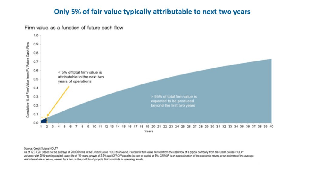
The only “drawback” I see here is that the valuation of a company is not as dependent on the next five years of cash flows as it is on the terminal growth rate. Most DCFs assume that the company will be a going concern and therefore discount cash flows to infinity. The interesting thing is that many investors spend far too much time forecasting the free cash flows of the next five years rather than spending significant time on the topics of durability and growth runways, both arguably much more important to judge the valuation of a company.
(2) The terminal growth rate
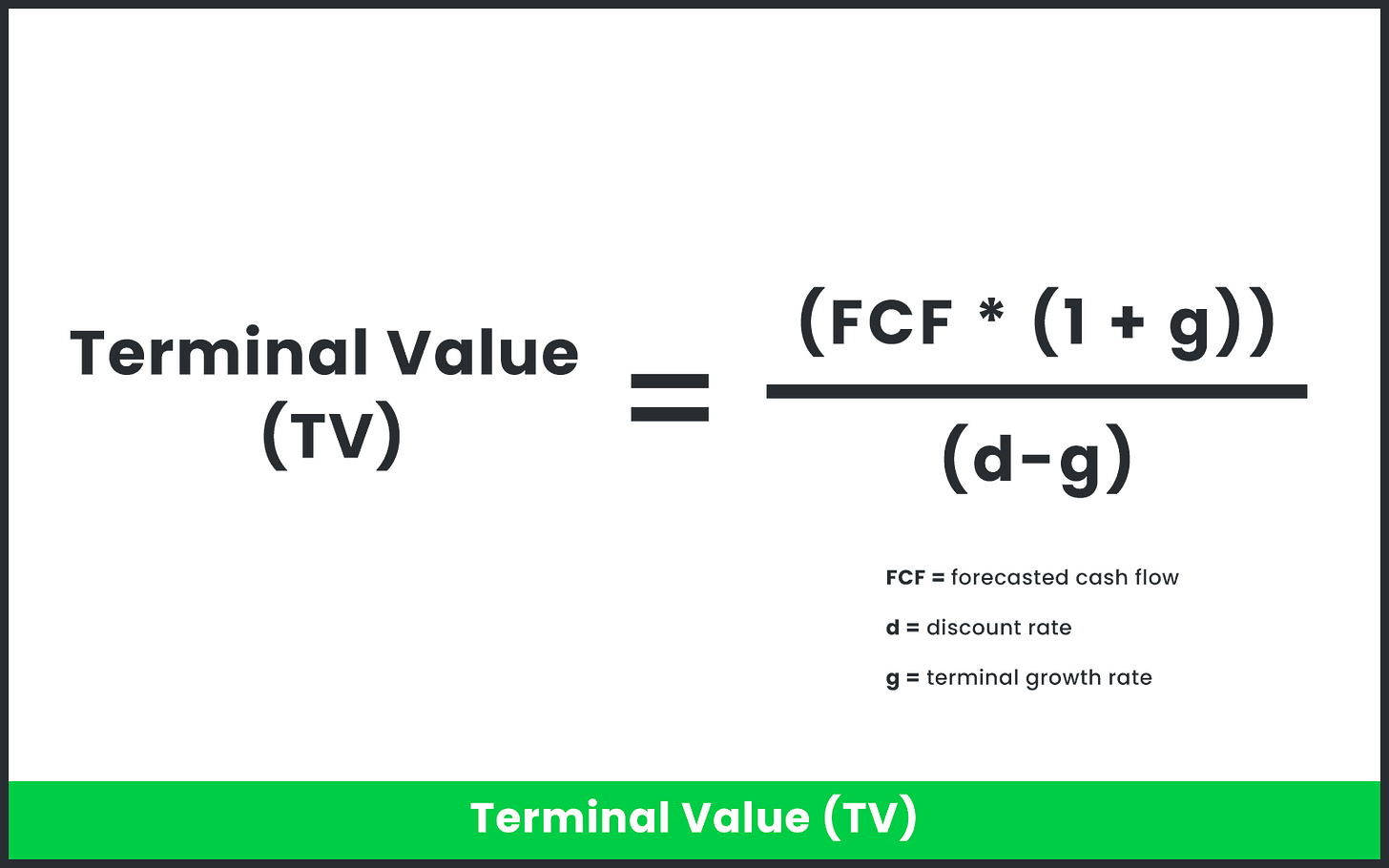
Once we get to the end of our forecasting period (could be 5, 10, or 20 years), we must assess the terminal value of the company. The terminal value will be calculated dividing the cash flow of the year t + 1 (where t is the ending year of the forecasting period) by the difference between the discount rate and the terminal growth rate. As most of the value relies on the terminal value (remember, for any company that we deem to be a going concern), our assumptions around these two variables are key.
The terminal growth rate is the rate at which we expect the company will grow beyond the forecast period into infinity. It’s nominal and we should not set it above nominal GDP growth because that theoretically means that a company could become larger than the global economy over time. The terminal growth rate, when used conservatively, penalizes the really durable businesses. The reason is that if we drop the growth rate of a durable business in the fifth year to a terminal rate, we would probably be underestimating its terminal value. Durable companies can grow above their terminal growth rates far longer than a 5-year DCF model might portray, which is why they tend to appear optically overvalued only to continue outperforming expectations (unsurprisingly, I have also written an article about this: ‘What Makes Quality Undervalued’).
This is undoubtedly a drawback, but as my good friend Drew Cohen from Speedwell Memos once told me, a possible solution might be to expand the forecasting period so long as the company has high visibility and one can have reasonable confidence in forecasting, say, 20 years out. This is what I have done in my Hermès valuation model, which subscribers can access here.
(3) The discount rate
The discount rate is the other key variable in determining not only the terminal value of a business but also its overall intrinsic value. Unlike the terminal growth rate, which is only present in the terminal value calculation, the discount rate is the rate used to discount all cash flows. Obviously, it’s impact on the discounting of the terminal value is much more significant than on the discounting of the next 5 years of cash flows.
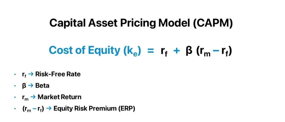
Common finance knowledge states that we should use the Weighted Average Cost of Capital (also known as WACC) as the discount rate. This metric is a weighted average of the different financing options available to a company, namely equity and debt. The cost of debt is fairly straightforward to calculate, but to calculate the cost of equity we need to use something called the Capital Asset Pricing Model or CAPM. I’ll leave here the formula, but I won’t explain it because I don’t use it:
This is what theory states, but I tend to use my required rate of return as the discount rate. In many cases, this will be pretty similar to WACC because I hold several companies with no debt, but when a company has debt, it’ll probably be significantly higher than what the WACC would’ve been (which is good because it’s more conservative). I’ll change my discount rate according to the risk I see in the company. For example, the discount rate I use for Nintendo is higher than the one I use for Hermes due to the diverging visibility and predictability of both businesses.
As mentioned above, the most interesting thing about the DCF is how much time people spend on the first of these three variables (the cash flows of the next 5 years) when it’s the one that impacts the valuation the least. This can also be seen as a drawback of the DCF model: it’s very sensitive to changes in the terminal growth rate and the discount rate, both of which are pretty subjective.
4. The inverse DCF
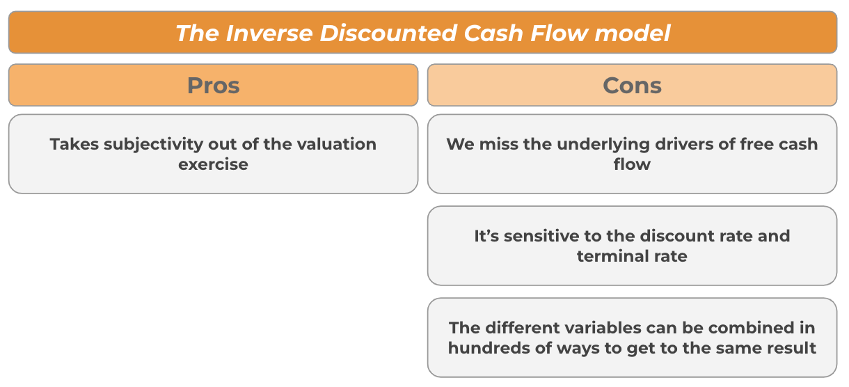
The inverse DCF is simple to explain once we know how a regular DCF works. In a regular DCF we must include all the inputs to get to an intrinsic value for a given company. The inverse DCF works backwards and tries to find what is currently priced into the current valuation. One starts with the current stock price and aims to find out what FCF growth rate and terminal growth rate the market is assuming for a given discount rate (this is our “only” real input). Once we get the output of the inverse DCF, the goal is to judge whether the market's expectations are reasonable or not (there’s a lot of qualitative work required here, as you might have imagined), and, therefore, whether the stock is undervalued, overvalued, or fairly valued.
The main advantage of this method is that it takes away some of the subjectivity around the inputs, but the drawback is that it still remains sensitive to the terminal and discount rates. There are many combinations of the three variables that I explained above that can take us to a given stock price, and it’s pretty much impossible to know if what we find out is exactly what the market is pricing in. The other drawback is that, once we get to the FCF CAGRs required to “make the stock work,” we might not appropriately understand its underlying drivers.
My preferred method: working backwards from an inverse DCF
Up until here, I’d say that the inverse DCF is the method that most resonates with me, although it has a significant drawback. The most important drawback of these in my opinion, is the opacity of the FCF growth drivers, which I have found a “workaround” for.
I now do an inverse DCF in two steps. First, I find the required free cash flow growth rates that are implied in the price just as I discussed above. Once I have these, I work through assumptions regarding…
Revenue growth
Margin expansion
Cash conversion
Capex
…that lead me to those implied Free Cash Flow growth rates. Of course, there are hundreds of combinations that can work, but the goal is to end up with something reasonable. For example, if a company is currently undergoing a significant capacity expansion plan, it would make little sense for me to use Capex leverage as a driver of free cash flow growth over the coming years. But, why is this useful? Because (a) we get more information, and (b) we can see if the numbers are normalized.
I’ll share here a brief example of where this can come in handy. Last year I was building my inverse DCF for Zoetis, and the model spit out pretty steep required FCF growth rates. At first sight, these might have appeared to be unachievable for a company like Zoetis. However, after digging deeper by working on the underlying drivers, I found out that cash conversion had been penalized due to inventory buildup, something that was expected to be temporary. This meant that, to reach those FCF growth figures, the company did not actually have to grow revenue at an above-average pace because much of that growth would come from a return to normal in terms of cash conversion. That’s precisely what we have seen play out: free cash flow conversion has largely normalized, and free cash flow has grown significantly ahead of revenue (this, by the way, also happened in 2016):
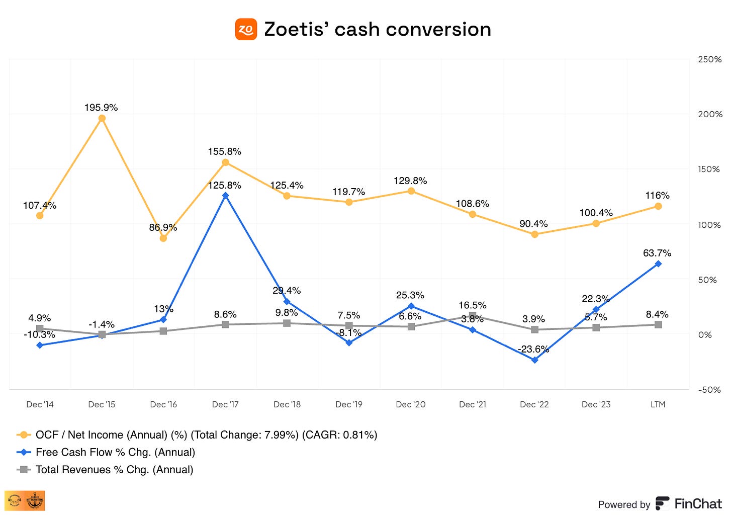
If I had ignored the underlying drivers of free cash flow by just focusing on the output of the inverse DCF, I would’ve most likely concluded that Zoetis was significantly overvalued because those growth rates were unachievable for the company. After going through the underlying drivers, I concluded that the growth rates were achievable because they came to a large extent from a return to a normalized environment.
This method has the same pros and cons than the inverse DCF with the only exception that we must explicitly work through the underlying drivers and therefore, it’s less opaque.
Conclusion
I hope this article was useful in understanding the main pros and cons of the different valuation methods (or how I view these). I don’t want to end this article without making two caveats.
First, more complex valuation methods can give us a false sense of security, but if the reasoning is sound and we control for the drawbacks, any valuation method is useful in assessing the value of a company.
Secondly, valuing a company requires making future projections which require current numbers plus a very good understanding of the underlying drivers of a company. Many people jump to valuation conclusions without having researched a company enough, and that can be very dangerous. Valuation is of utmost importance, but it should always come last in the research process or else it will be blind guessing. It’s unlikely we’ll get the numbers right even if we know a lot about a company, but we should at least make an educated guess rather than a blind one.
In the meantime, keep growing!
Disclaimer: Leandro holds shares of several companies discussed in this article, which does not constitute formal advice or recommendation; it was uploaded with informational purposes only. Do your own due diligence.


Brilliant Leandro, as always